

Introduction 🔗
In this blog post, we will explore fundamental object detection technique called Histograms of Oriented Gradients (HOGs). Interestingly, I came across this method in a sort of unconventional way, that is while browsing the comment section of a completely unrelated YouTube video. What began as a casual scroll quickly turned into an unexpected discovery, sparking my curiosity to dive deeper into this subject. After having done a reasonable amount of exploring the concepts, applications, and implementation, I am excited to share my findings with you.
While the primary focus will be on understanding HOGs and their role in object detection, we will also take things a step further by applying this knowledge to a practical task: classifying some of the most common flowers found in the UK (17 flowers dataset). This choice of application is not arbitrary. After doing a quick search on Google Scholar and the Web, I noticed that while both HOG features and color histograms have been used individually or in combination with other techniques for plant and flower classification, there are relatively few articles that specifically explore the combination of HOG and color histograms for this purpose.
This pairing is particularly compelling because it allows us to capture both the shape and structural details of the flowers (by means of HOGs) alongside their rich and varied color patterns (via color histograms).
We will begin by exploring the implementation details with the help of visual elements (animations, images) and then proceed to build the functionality from scratch without relying on any third-party libraries. Finally, we will wrap up by creating the flower classifier.
By the time you finish this post, we will have built an image classifier that achieves an impressive 94% test accuracy!
Histograms of Oriented Gradients 🔗
Introduced by Navneet Dalal and Bill Triggs in 2005. It became particularly famous for human detection applications and served as a foundational technique that influenced many modern computer vision approaches.
Histograms of Oriented Gradients are like edge-detectors but on steroids, they not only extract gradients (that tell use information about pixel intensity), but also orientation (the direction of the change in pixel intensity). These gradients and orientations are computed for local regions of an image, often called cells, and for each cell a histogram is calculated. Hence the name Histograms of Oriented Gradients. Details on this are covered in the following sections.
Dataset in question
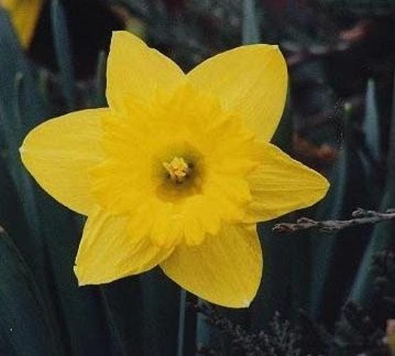
The following image showcases a sample from our dataset which we will use throughout this post to illustrate key concepts. The example features a Daffodil flower, one of the most recognizable and vibrant blooms commonly found in the UK.
Pre-processing
As per any task in computer vision, or machine learning in general, we should start of by applying pre-processing steps. The original paper (that studied HOGs performance for Human detection) mentions the following, citing.
Our 64×128 detection window includes about 16 pixels of margin around the person on all four sides.
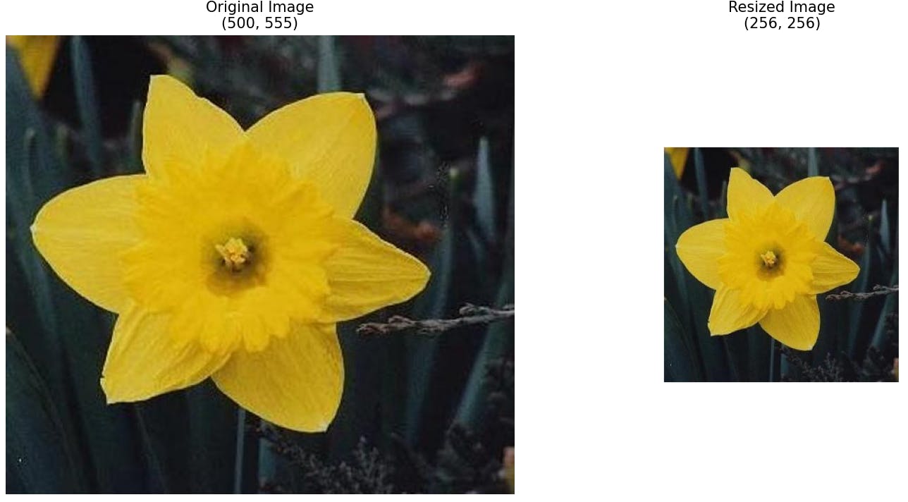
The exact 64×128 size seems to have been chosen empirically, for the specific task in hand, to include a reasonable margin around the pedestrian while matching the general scale of pedestrians in their dataset. The paper does not provide a theoretical justification for this particular window size, therefore for our task, considering the varied shapes and close-up nature of the flower images, I opted to resize all images to a uniform size of 256×256 pixels, ensuring consistency and better suitability for flower classification.
Gradient computation
The succeeding step is to compute vertical and horizontal gradients, that is the pixel intensity changes both in x and y directions. Gradient computation is a crucial step in the HOG feature extraction process. To calculate the gradients, we will not re-invent the wheel, rather we use specially selected kernels whose main purpose is to detect such pixel intensity changes in either of directions. The most commonly used kernels for this purpose are the [-1, 0, 1] kernel for the horizontal gradient and its transpose, [-1, 0, 1]ᵀ, for the vertical gradient. To apply these kernels, they are slid across the image in a process called convolution. At each pixel location, the kernel is centered, and the pixel values are multiplied by the corresponding kernel values. The results are then summed up to obtain the gradient value at that particular pixel. This process is repeated for every pixel in the image, resulting in two gradient maps – one for the horizontal gradient and another for the vertical gradient.
Important note! Before performing this step, a decision must be made about whether to convert the input image to grayscale or keep it in its original multichannel form. If the image is converted to grayscale, the gradient computation is straightforward and performed on a single channel. However, if the image remains multichannel, gradients are computed separately for each channel, resulting in multiple gradient maps (one for each channel). Keeping the color information can lead to improved performance later down the line.
 The animation demonstrates this process with horizontal kernel, but the same idea would apply for horizontal gradient computation (on a small patch extracted from the sample image).Notably, as visible in animation, regions with significant changes in pixel intensity tend to exhibit larger gradient values. These areas correspond to edges, boundaries, or transitions within the image. In our case, these changes often occur due to the distinct edges of flower petals, where the shape of the petal creates sharp contrasts against the background or adjacent petals.
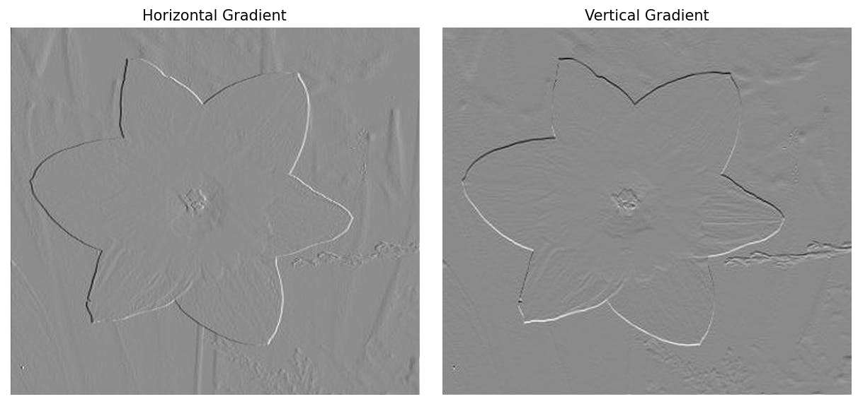 Final gradient (horizontal and vertical) gradient computation. Fun fact, that might seem counterintuitive at first, but the horizontal kernel detects vertical changes, similarly, the vertical kernel is aligned vertically, but it detects horizontal changes
Magnitude and orientation computation
With the gradient computation in place, we can now finally determine the magnitude value for each pixel. Now you might wonder, why bother calculating magnitude when we already have the horizontal and vertical gradients? The answer is plain and simple: relying on just one gradient can miss the bigger picture, especially for edges that are angled or diagonal. To fully capture the strength of an edge, we combine the horizontal and vertical gradients using the good old Pythagorean theorem. Might have sounded harder than it really is, however it is as elementary as applying a bit of high school math.
Important note! I chose to preserve all of the RGB channels of the image, therefore the final magnitude is the largest one amongst all of the image channels for a particular pixel.

After calculating the magnitude of the gradient, the next step is to compute the orientation of the gradient at each pixel. The orientation represents the direction of the edge and provides additional information about the structure and shape of the objects in the image.
The resulting angle is then typically converted to degrees for easier interpretation, in addition a crucial decision must be made regarding whether to keep the angle signed (-180° to 180°) or unsigned (0° to 360°). In the original paper the authors experimented with various approaches and found that for human detection, using unsigned gradients over angles of 0° to 180° provided the best performance. I experienced no perceptible accuracy improvements using either of the approaches for flower classification.
Histogram computation
The next step in HOG feature extraction pipeline is to create histogram representations of these gradients. To begin, the image is to be divided into smaller, local regions called 'cells', as we remember from introduction.
In the original paper, the authors used 8x8 pixel cells, their justification was that 'relatively coarse spatial quantization suffices (8×8 pixel cells / one limb width)'. This reasoning suggests that the cell size should be chosen to roughly correspond to the size of meaningful parts or features of the objects being detected, which aligns with my discoveries, more specifically in my experiments with flower classification, I found that using a larger cell size of 16×16 provided better results for the task in hand. It is important to emphasize that the cell size can be adjusted based on the characteristics of the objects being detected and the resolution of the images. When selecting the cell size, it is significant to ensure that the cells evenly divide the image. In other words, the image dimensions should be divisible by the cell size without leaving any remainder, which ensures that all cells have the same size and that there are no partial or incomplete cells at the edges of the image. For example, as in our case the images are resized to have dimensions of 256×256 pixels, we could have chosen cell sizes of 8×8, 16×16, 32×32, or 64×64, as all of these sizes evenly divide the image. On the other hand, lets say if the image has dimensions of 150×150 pixels, a cell size of 16×16 would not be suitable, as it would result in uneven cells at the image boundaries.
 Illustration of target image being divided into 16x16 cells
Great, now that we have divided our image into cells, we end up with 16×16×2 = 512 total values for each cell. This comes from the fact that each cell consists of 16×16 = 256 pixels, and for each pixel, we have calculated two key values - magnitude and orientation. With these values in hand, we can now move on to the more exciting part of calculating the histograms of oriented gradients for each cell!
A histogram is a visual representation of the distribution of quantitative data. To construct a histogram, the first step is to "bin" the range of values— divide the entire range of values into a series of intervals—and then count how many values fall into each interval
In HOGs histograms represent the distribution of gradient orientations within a particular cell. The gradient orientations are typically quantized into a fixed number of bins, commonly 9, as suggested in the original paper: 'increasing the number of orientation bins improves performance significantly up to about 9 bins.' With 180° divided into 9 bins, each bin covers a span of 20°. The construction of the histogram is the following, we directly take each pixels gradients magnitude and add it to the corresponding orientation bin. The resulting histogram for each cell provides a compact representation of dominant edges while abstracting away the exact spatial locations of the gradients within the cell.
 Illustrative animation of the histogram creating process by 'binning' (on a 6x6 patch for visualization purposes)
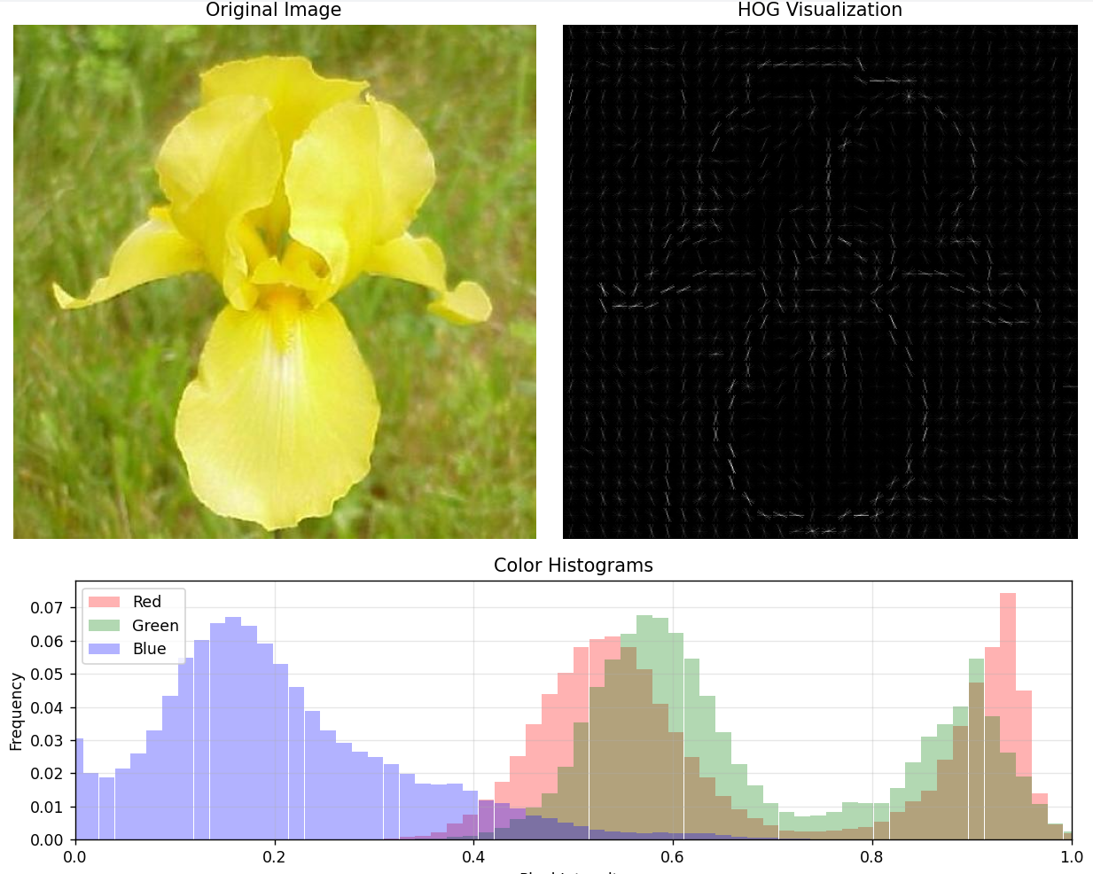
 Resulting visualization constructed from histograms
Block normalization
We have arrived at the final finishing touch for HOG computation, which is to perform block normalization. Block normalization is a crucial technique used to further improve invariance of the HOG to changes in illumination and contrast.
The need for block normalization arises from the fact that the gradient magnitudes can vary significantly across different regions of an image due to variations in lighting conditions, shadows, and local contrast. The above mentioned variations can adversely affect the performance of a classifier because of the inconsistent object description. Block normalization helps to mitigate such an issue by normalizing the histogram values across larger spatial regions called 'blocks'.
A block is a group of adjacent cells, typically 2×2 or 3×3 cells, that are treated as a single unit for the means of normalization. In simple words, this means that we concatenate 4 or 9 histograms together in one large list (respectively, forming 4×9 = 36 or 9×9 = 81 histogram values). The block size is usually larger than the cell size to capture a wider spatial context. The blocks are overlapped, meaning that each cell contributes to multiple blocks. The normalization procedure involves computing L2 normalization (essentially normalization based off of Euclidean distance) or L2-Hys normalization of the block. The study shows that both methods display close performance.
After block normalization is finished we have the final feature set that describes our object, the authors in the paper introduce them as HOG descriptors: 'We will refer to the normalized descriptor blocks as Histogram of Oriented Gradient (HOG) descriptors'.
 Illustration of block normalization process. The final feature count is 15×15×4×9 = 8100 (256/32-1 = 15 blocks that fit width and height wise, each block is made up of 4 cells, each cell has 9 histogram values)
Important note! While raw histograms create intuitive visualizations of gradient directions, the normalized features are essential for machine learning tasks. Visualizing normalized features is less common since they represent abstract, high-dimensional block-wise patterns optimized for classification rather than human interpretation.
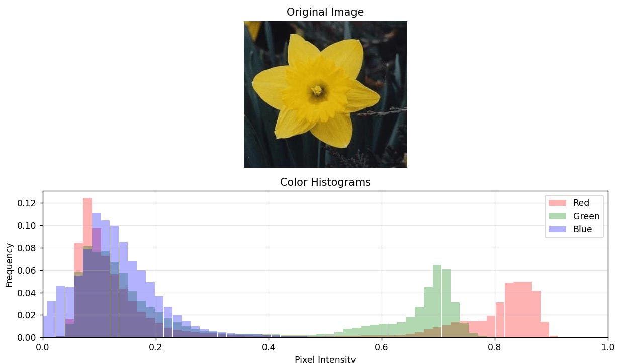
Color histograms 🔗
Although color histograms are not the main focus of this blog post, they do however expand our feature space with additional valuable characteristics. The process of creating color histograms closely mirrors the approach used for HOG. Here, instead of gradients, we 'bin' the pixel values from each image channel separately based on intensity ranges. In result we are left with 3 histograms, each for Red, Green and Blue channels, that provide a detailed representation of the color distribution withing the image. For the task of flower classification I found that 64 bins per channel yielded the highest performance enhancement, and any additional increase had little to no effect.
Code implementation 🔗
There are countless libraries that implement the above discussed functionality for us, however, I believe implementing it yourself adds that extra layer of understanding and truly solidifies the concept. In the first subsection I present you a straightforward hands on implementation that is easy to follow. In the second subsection we will walk through an implementation that uses third party libraries that have much more optimized solution utilizing smart matrix multiplications - this is the recommended choice for practical applications.
Building it ourselves
pip install numpy Pillow matplotlib scipy
The following code demonstrates how to implement HOG feature extraction from scratch using Python.
This implementation is encapsulated in a HOGExtractor class, which:
- Initializes Parameters: Sets up image size, cell size, block size, and the number of orientation bins required for HOG computation
- Loads and Preprocesses the Image: Handles resizing and normalization to ensure consistent input
- Computes Gradients: Uses kernels to calculate horizontal and vertical gradients, from which gradient magnitudes and orientations are derived
- Builds Cell Histograms: Divides the image into smaller regions (cells) and computes a histogram of gradient orientations for each region
- Performs Block Normalization: Slides across overlapping blocks of cells and performs normalization
- Generates the Final Descriptor: Concatenates all normalized block histograms into a feature vector that represents the image and objects inside of it
                    import numpy as np
from PIL import Image, ImageDraw
import matplotlib.pyplot as plt
from scipy.signal import convolve2d

class HOGExtractor:
    def __init__(self, image_size=(256, 256), cell_size=(16, 16), block_size=(2, 2), band_count=9):
        self.IMAGE_RESIZE_SIZE = image_size
        self.CELL_SIZE = cell_size
        self.BLOCK_SIZE = block_size
        self.BAND_COUNT = band_count
        self.BIN_WIDTH = 180 / band_count

        # Sobel operators for gradient computation
        self.horizontal_kernel = np.array([[-1, 0, 1]])
        self.vertical_kernel = np.array(self.horizontal_kernel.T)

        # Initialize computed attributes
        self.input_image = None
        self.resized_image = None
        self.gradient_magnitude = None
        self.gradient_orientation = None
        self.cell_histograms = None
        self.hog_descriptor = None

    def _load_image(self, pil_image):
        # The authors of HOG found an increase in accuracy
        # by taking into consideration all RGB channels, however we convert the image to grayscale for convenience of this example
        self.input_image = pil_image.convert('L')
        self.resized_image = np.array(self.input_image.resize(self.IMAGE_RESIZE_SIZE))
        self.resized_image = self.resized_image.astype(float)
        # Normalize the image pixel values to [0, 1]
        self.resized_image = (self.resized_image - self.resized_image.min()) / (self.resized_image.max() - self.resized_image.min())

    def _compute_gradients(self):
        # Apply sobel kernels using convolution
        # 'same' property ensures that the output has the same dimensions as the input image by automatically adding appropriate padding
        horizontal_gradient = convolve2d(self.resized_image, self.horizontal_kernel, mode='same')
        vertical_gradient = convolve2d(self.resized_image, self.vertical_kernel, mode='same')

        # Calculate gradient magnitude and orientation
        self.gradient_magnitude = np.sqrt(horizontal_gradient**2 + vertical_gradient**2)
        self.gradient_orientation = np.arctan2(vertical_gradient, horizontal_gradient) * (180 / np.pi) % 180

    def compute_cell_histograms(self):
        # Calculate number of cells in each dimension
        cells_y = self.IMAGE_RESIZE_SIZE[1] // self.CELL_SIZE[1]
        cells_x = self.IMAGE_RESIZE_SIZE[0] // self.CELL_SIZE[0]

        # Initialize histogram array for all cells
        self.cell_histograms = np.zeros((cells_y, cells_x, self.BAND_COUNT))

        # Compute histograms for each cell
        for y in range(cells_y):
            for x in range(cells_x):
                # Get current cell coordinates
                y_start = y * self.CELL_SIZE[1]
                y_end = (y + 1) * self.CELL_SIZE[1]
                x_start = x * self.CELL_SIZE[0]
                x_end = (x + 1) * self.CELL_SIZE[0]

                # Get magnitudes and orientations for current cell
                cell_magnitudes = self.gradient_magnitude[y_start:y_end, x_start:x_end]
                cell_orientations = self.gradient_orientation[y_start:y_end, x_start:x_end]

                # Create histogram for current cell
                histogram = np.zeros(self.BAND_COUNT)

                # Go over each pixel in the cell
                for i in range(self.CELL_SIZE[1]):
                    for j in range(self.CELL_SIZE[0]):
                        orientation = cell_orientations[i, j]
                        magnitude = cell_magnitudes[i, j]

                        # Compute bin index for current orientation, and add magnitude to corresponding bin
                        bin_index = int(orientation // self.BIN_WIDTH)
                        histogram[bin_index] += magnitude

                self.cell_histograms[y, x] = histogram

    def compute_hog_descriptor(self):
        # Calculate number of blocks
        cells_y = self.IMAGE_RESIZE_SIZE[1] // self.CELL_SIZE[1]
        cells_x = self.IMAGE_RESIZE_SIZE[0] // self.CELL_SIZE[0]
        blocks_y = cells_y - self.BLOCK_SIZE[0] + 1
        blocks_x = cells_x - self.BLOCK_SIZE[1] + 1

        # Initialize final HOG descriptor
        hog_descriptor = []

        # Slide the block window across cells
        for y in range(blocks_y):
            for x in range(blocks_x):
                # Get histograms for current block (2x2 cells)
                block_histograms = []
                for cell_y in range(self.BLOCK_SIZE[0]):
                    for cell_x in range(self.BLOCK_SIZE[1]):
                        cell_histogram = self.cell_histograms[y + cell_y, x + cell_x]
                        block_histograms.extend(cell_histogram)

                # Normalize block using L2 norm
                # Small epsilon value prevents division by zero
                block_histograms = np.array(block_histograms)
                l2_norm = np.sqrt(np.sum(block_histograms ** 2) + 1e-6)
                normalized_block = block_histograms / l2_norm

                # Add normalized block histograms to final descriptor
                hog_descriptor.extend(normalized_block)

        self.hog_descriptor = np.array(hog_descriptor)
        return self.hog_descriptor

    def extract_features(self, pil_image):
        self._load_image(pil_image)
        self._compute_gradients()
        self.compute_cell_histograms()
        return self.compute_hog_descriptor()

    def visualize(self):
        self._visualize_hog()

    def _visualize_hog(self):
        # Calculate dimensions
        cells_y = self.IMAGE_RESIZE_SIZE[1] // self.CELL_SIZE[1]
        cells_x = self.IMAGE_RESIZE_SIZE[0] // self.CELL_SIZE[0]

        # Create visualization
        vis_image = Image.new('RGB', self.IMAGE_RESIZE_SIZE, 'black')
        draw = ImageDraw.Draw(vis_image)

        cell_height, cell_width = self.CELL_SIZE
        line_length = min(cell_height, cell_width) // 2

        # Draw lines using raw cell histograms directly
        for y in range(cells_y):
            for x in range(cells_x):
                # Use raw cell histograms instead of normalized ones
                raw_histogram = self.cell_histograms[y, x]
                self._draw_cell_visualization(draw, x, y, cell_width, cell_height,
                                        line_length, raw_histogram)

        self._show_visualization(vis_image, 'Raw HOG Visualization')

    # Private helper  function to draw cell visualization
    def _draw_cell_visualization(self, draw, x, y, cell_width, cell_height, line_length, histogram):
        cell_center_y = (y + 0.5) * cell_height
        cell_center_x = (x + 0.5) * cell_width

        for orientation_bin in range(self.BAND_COUNT):
            orientation = orientation_bin * (180 / self.BAND_COUNT)
            magnitude = histogram[orientation_bin]


            radian = np.deg2rad(orientation)
            dx = line_length * np.cos(radian) * magnitude / np.max(histogram)
            dy = line_length * np.sin(radian) * magnitude / np.max(histogram)

            draw.line([
                (cell_center_x - dx, cell_center_y - dy),
                (cell_center_x + dx, cell_center_y + dy)
            ], fill='white', width=1)

    # Private helper function to show visualization
    def _show_visualization(self, vis_image, title):
        plt.figure(figsize=(10, 15))
        plt.subplot(311)
        plt.title('Original Image')
        plt.imshow(self.input_image, cmap='gray')

        plt.subplot(312)
        plt.title(title)
        plt.imshow(vis_image)

        plt.tight_layout()
        plt.show()
Leveraging the Pros
pip install scikit-image numpy matplotlib
Why Use a Library? While implementing HOG from scratch deepens understanding, third-party libraries like scikit-image offer optimized implementations (from my testing the feature extraction process was approximately 10 times faster)
                    from skimage.feature import hog
from skimage.transform import resize
import numpy as np
import matplotlib.pyplot as plt

class HOGExtractor:
   def __init__(self, image_size=(256, 256), cell_size=(16, 16), block_size=(2, 2), band_count=9):
        self.image_size = image_size
        self.input_image = None
        self.cell_size = cell_size
        self.block_size = block_size
        self.band_count = band_count

    def extract_features(self, image):
        self.input_image = image
        img_array = np.array(image)
        img_array = resize(img_array, self.image_size)

        features, hog_image = hog(
            img_array,
            orientations=self.band_count,
            pixels_per_cell=self.cell_size,
            cells_per_block=self.block_size,
            visualize=True,
            channel_axis=-1
        )
        self.hog_image = hog_image
        return features

    def visualize(self):
        if self.input_image is None or self.hog_image is None:
            return

        plt.figure(figsize=(10, 5))

        plt.subplot(121)
        plt.title('Original Image')
        plt.imshow(self.input_image)
        plt.axis('off')

        plt.subplot(122)
        plt.title('HOG Visualization')
        plt.imshow(self.hog_image, cmap='gray')
        plt.axis('off')

        plt.tight_layout()
        plt.show()
                    import numpy as np
import matplotlib.pyplot as plt

class ColorHistogramExtractor:
    def __init__(self, bins=256, channels=3):
        self.bins = bins
        self.channels = channels
        self.image = None
        self.histograms = None
        self.colors = ['red', 'green', 'blue']
        self.channel_names = ['Red', 'Green', 'Blue']

    def load_image(self, pil_image):
        self.image = np.array(pil_image)
        return self

    def extract_features(self, image_array=None, normalize=True):
        if image_array is not None:
            self.load_image(image_array)

        self.histograms = []
        for channel in range(self.channels):
            histogram, _ = np.histogram(
                # Selects all pixels for a specific color channel (R, G, or B) using numpy's ellipsis notation
                # and flattens the 2D array of pixel values into a 1D array
                self.image[..., channel].ravel(),
                bins=self.bins, # divides the range into equal-width bins
                range=(0, 256)
            )

            if normalize:
                histogram = histogram / histogram.sum()

            self.histograms.append(histogram)

        return np.concatenate(self.histograms)

    def visualize(self):
        plt.figure(figsize=(10, 6))

        # Plot original image
        plt.subplot(2, 1, 1)
        plt.title('Original Image')
        plt.imshow(self.image)
        plt.axis('off')

        # Plot histograms as bars
        plt.subplot(2, 1, 2)
        plt.title('Color Histograms')

        x = np.linspace(0, 1, self.bins)  # Normalized x-axis [0,1]
        bar_width = 1.0 / self.bins

        for channel in range(self.channels):
            plt.bar(x, self.histograms[channel],
                color=self.colors[channel],
                label=self.channel_names[channel],
                alpha=0.3,
                width=bar_width)

        plt.xlabel('Pixel Intensity')
        plt.ylabel('Frequency')
        plt.legend()
        plt.grid(True, alpha=0.3)
        plt.xlim(0, 1)  # Set x-axis limits to [0,1]

        plt.tight_layout()
        plt.show()
Flower classifier 🔗
In this last section, we implement a flower classifier using HOG features, color histograms, and a Random Forest Classifier. The classifier is trained on the above mentioned 17 Category Flower Dataset, which consists of 17 flower classes. The following is a short overview of the workflow:
- Feature Extraction: We use a combination of HOG features (to capture shape and texture information) and color histograms (to leverage color distribution in the images). These features provide a rich representation of each image containing a flower
- Training and Testing Splits: The original dataset was split into 3 different training, validation and test sets. For our use case all of the different training sets and test sets were combined to form a complete training and testing set, containing 2040 and 1040 samples respectively
- Model Pipeline: A pipeline is constructed with a Standard Scaler to normalize the feature values to a similar scale in order to remove any potential bias and a Random Forest Classifier
pip install scikit-learn scipy numpy pillow tqdm
                    from hog import HOGExtractor
from color_histogram import ColorHistogramExtractor
from sklearn.ensemble import RandomForestClassifier
from sklearn.preprocessing import StandardScaler
from sklearn.pipeline import Pipeline
import os
import scipy.io
import numpy as np
from PIL import Image
from tqdm import tqdm

# Constants
IMAGE_SIZE = (256, 256)
BIN_COUNT = 9

# Load dataset splits
datasplits = scipy.io.loadmat('datasplits.mat')
dataset_path = './17flowers/jpg'
image_files = sorted([f for f in os.listdir(dataset_path) if f.endswith('.jpg')])

# Initialize feature extractors
hog_extractor = HOGExtractor(image_size=IMAGE_SIZE)
color_extractor = ColorHistogramExtractor(bins=BIN_COUNT)

def load_and_extract_features(indices):
    features_list = []
    labels = []

    for idx in tqdm(indices, desc="Extracting features"):
        # Load image
        img_path = os.path.join(dataset_path, image_files[idx-1])
        img = Image.open(img_path)

        # Create label (17 classes, indexed 0-16)
        label = (idx-1) // 80  # Each class has 80 images
        labels.append(label)

        # Extract features
        hog_features = hog_extractor.extract_features(img)
        color_features = color_extractor.extract_features(img)

        # Combine features
        combined_features = np.concatenate([hog_features, color_features])
        features_list.append(combined_features)

    return np.array(features_list), np.array(labels)

# The original dataset has 3 training, testing, validation splits
# We combine all of the training and testing data into a single set
all_train_indices = np.concatenate([
    datasplits[f'trn{split}'].ravel()
    for split in range(1, 4)
])
all_test_indices = np.concatenate([
    datasplits[f'tst{split}'].ravel()
    for split in range(1, 4)
])

# Extract features for current split
X_train, y_train = load_and_extract_features(all_train_indices)
X_test, y_test = load_and_extract_features(all_test_indices)

pipeline = Pipeline([
    ('scaler', StandardScaler()),
    ('classifier', RandomForestClassifier(
        n_estimators=300,
        max_depth=50,
        min_samples_split=5,
        min_samples_leaf=2,
        max_features='sqrt',
        class_weight='balanced_subsample',
    ))
])

# Fit and evaluate
pipeline.fit(X_train, y_train)
train_accuracy = pipeline.score(X_train, y_train)
test_accuracy = pipeline.score(X_test, y_test)
print(f"Train accuracy: {train_accuracy:.3f}, Test accuracy: {test_accuracy:.3f}")
 The training accuracy of 1.0 (100%) with test accuracy of 0.946 (94.6%) indicates some overfitting, but it is not necessarily problematic in this case, because of the nature of Random Forests. Random Forests could achieve 100% training accuracy through their tree structure and ensemble nature, especially since the chosen model parameters create many deep trees, which eventually have reaching leaf nodes that contain samples from just one class.
Wrapping up 🔗
And that is a wrap! By now you should have a solid grasp of inner workings and/or implementation of HOG and how it can be combined with color histograms to build a feature-rich representation of images. These techniques are fantastic for tasks like object detection and classification. The Random Forest classifier performed pretty well on the flower dataset, but there is always room for improvement, maybe experimenting with other classifiers or tuning hyperparameters could get even better results.
For those interested in exploring more, Local Binary Patterns (LBP) is another powerful texture descriptor worth looking into. It is a simple yet effective technique that can complement HOG in certain scenarios.
Ultimately, the beauty of these methods lies in their adaptability. There is always more to uncover, more to discover, and sometimes the most interesting results come from just trying out new combinations!