Introduction
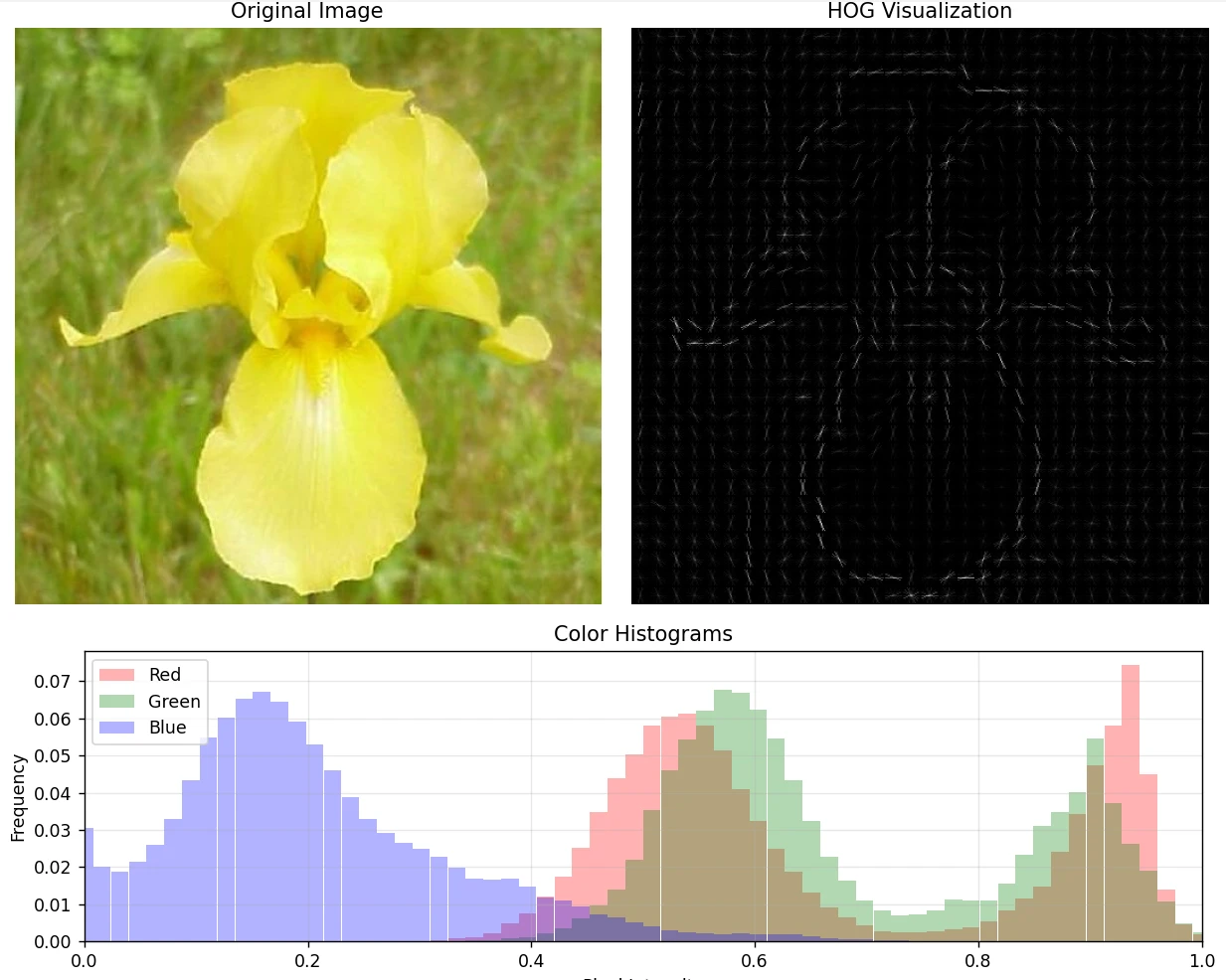
Histograms of Oriented Gradients (HOG) encode local image structure by aggregating gradient orientations over spatial regions. Originally introduced for human detection, HOG can remain a useful classical descriptor when object contours, texture, and local shape carry discriminative information.
Using the Oxford 17 Category Flower Dataset, this article traces HOG from pixel gradients to a normalized descriptor, then pairs it with RGB histograms. Flowers provide a useful example because their appearance depends on both local structure and color.
Histograms of Oriented Gradients
Introduced by Navneet Dalal and Bill Triggs in 2005, HOG describes an image through the locations and directions of changes in brightness. Strong changes often indicate visible boundaries; their orientations capture whether those boundaries are horizontal, vertical, or diagonal.
For each local region, or cell, HOG records both the strength of these changes and their orientation. The values are accumulated into orientation histograms and normalized across neighboring cells, producing a descriptor that preserves the arrangement of local structure while reducing sensitivity to illumination and contrast.
Dataset
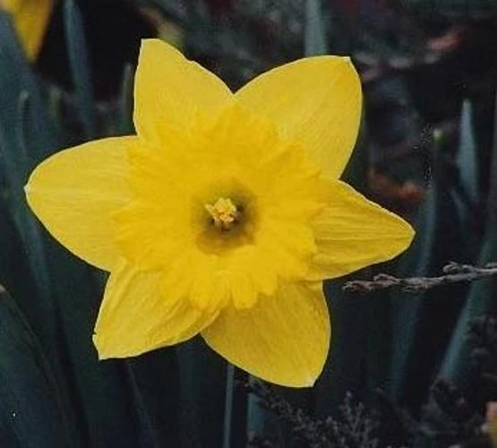
The Oxford dataset contains 17 flower categories with 80 images per category. It includes substantial variation in scale, pose, lighting, and background. A daffodil image from the dataset is used throughout the article to illustrate the individual stages of feature extraction.
Preprocessing
HOG requires a consistent spatial layout, so the first step is to resize each image to a fixed resolution. The original paper, which evaluated HOG for human detection, used a 64×128-pixel detection window with a margin around each subject:
Our 64×128 detection window includes about 16 pixels of margin around the person on all four sides.
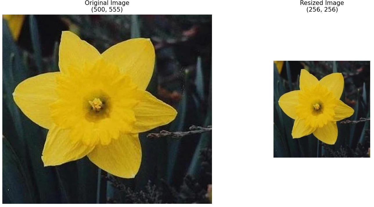
That resolution is specific to the scale and aspect ratio of pedestrians in the authors’ dataset. Flower images differ considerably in composition, so I resize them to 256×256 pixels. This preserves more local detail while ensuring that every image produces a descriptor of the same length.
Gradient computation
The next stage computes changes in pixel intensity along the horizontal and vertical axes. A finite-difference kernel, [-1, 0, 1], estimates the horizontal derivative, and its transpose (flipped version) estimates the vertical derivative. Convolving the image with both kernels produces two gradient maps containing the local rate of change along each axis.
Gradient handling differs between grayscale and multichannel images. A grayscale image produces one pair of gradient maps, while RGB gradients can be computed independently for each channel.
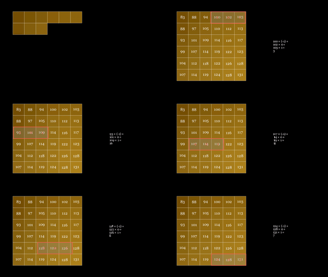
The animation demonstrates this process with a horizontal kernel on a small patch extracted from the sample image.
Regions with substantial changes in intensity produce larger gradient values. These commonly correspond to edges or boundaries. For example, the transition between a flower petal and its background.
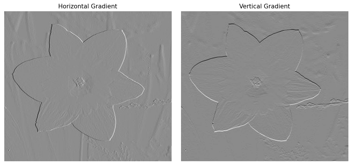
Final horizontal and vertical gradient computation. Counterintuitively, the horizontal kernel detects vertical changes, while the vertically aligned kernel detects horizontal changes.
Magnitude and orientation computation
The horizontal and vertical derivatives describe change along individual axes. Combining them with the Euclidean norm produces the gradient magnitude, which represents the overall strength of the local intensity change, including diagonal edges. Their ratio determines the orientation, or direction, of that change. For RGB input, the magnitude and orientation are taken from the channel with the strongest response at each pixel.


The orientation is usually expressed in degrees. HOG may use signed orientations over 0°-360° or unsigned orientations over 0°-180°. Dalal and Triggs found unsigned gradients more effective for human detection, so the implementation here follows that convention.
Histogram computation
The next stage divides the image into local regions called cells and summarizes the gradient orientations within each one. Dalal and Triggs used 8×8-pixel cells, observing that relatively coarse spatial quantization was sufficient for their detection task. Smaller cells preserve finer spatial detail but increase descriptor length, while larger cells provide a coarser representation. I use 16×16-pixel cells for the 256×256 flower images; the dimensions divide evenly without cropping or padding.
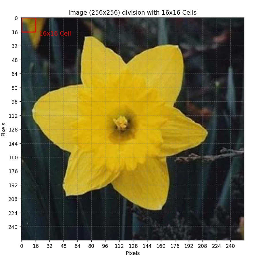
Illustration of the target image being divided into 16×16 cells.
Within each cell, orientations are quantized into a fixed number of bins. The original paper found that performance improved up to approximately nine orientation bins. Dividing the unsigned 0°-180° range into nine bins gives each bin a width of 20°.
Each pixel contributes its gradient magnitude to the relevant orientation bin. The resulting histogram represents the dominant local edge directions while abstracting away their exact pixel locations. Standard HOG implementations interpolate votes between neighboring bins.
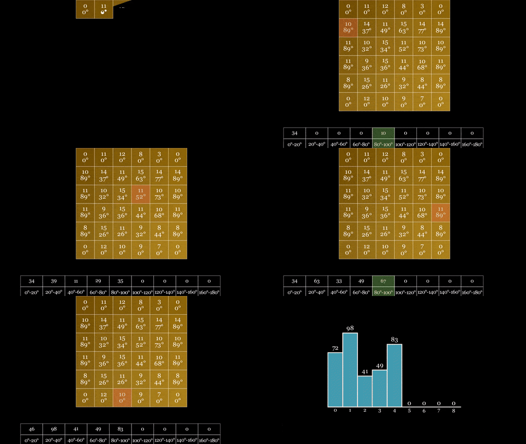
Illustrative animation of the histogram creation process by binning a 6×6 patch.
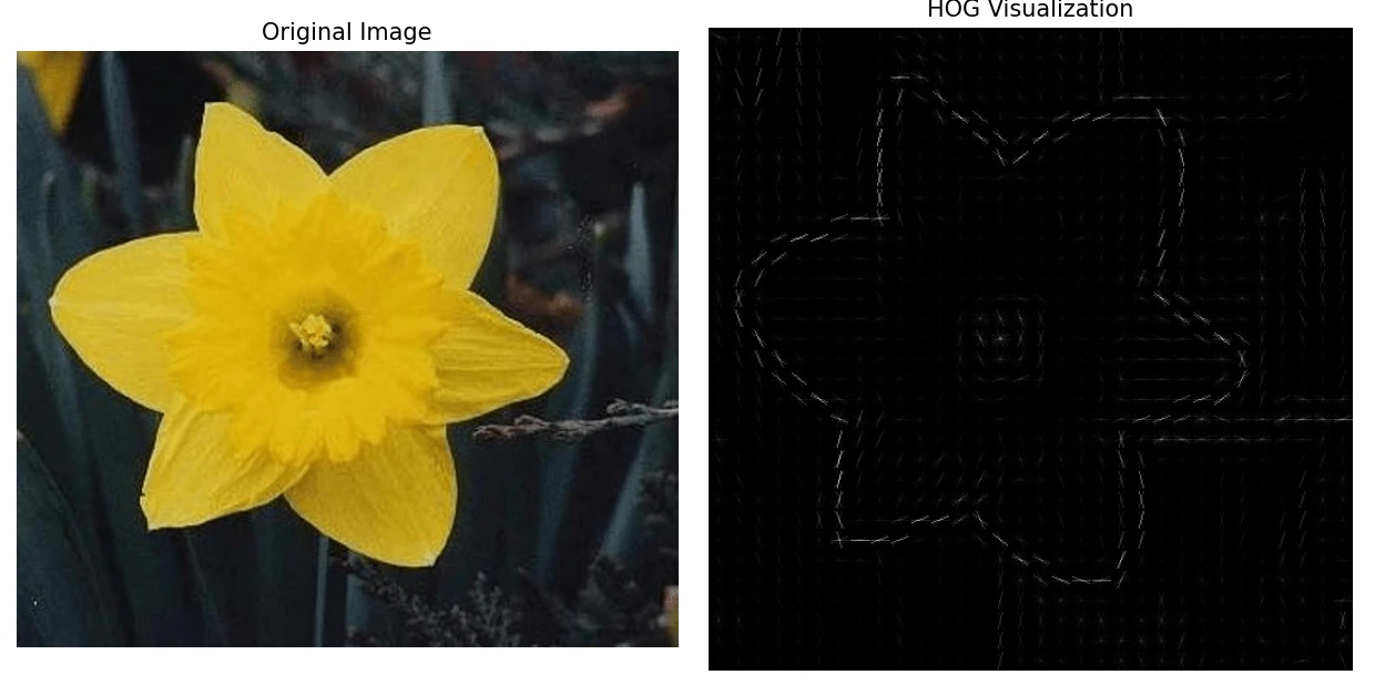
Block normalization
Gradient magnitudes vary with lighting, shadows, and local contrast. Block normalization reduces this sensitivity by normalizing histograms across groups of adjacent cells, commonly in a 2×2 or 3×3 arrangement. Four nine-bin histograms produce a 36-value block vector, while nine produce 81. The blocks overlap as they move across the image, so most cells contribute to multiple normalized vectors. Concatenating them produces the final HOG descriptor.
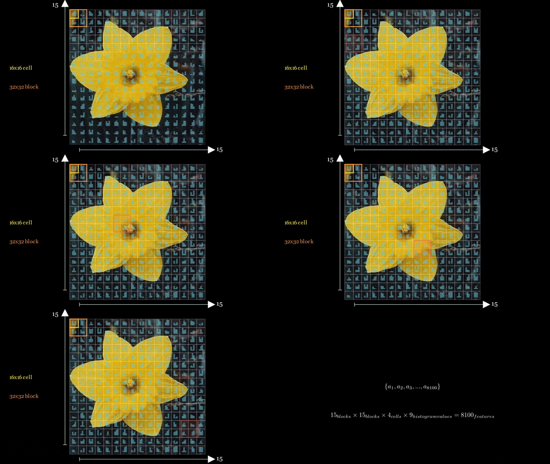
Illustration of block normalization. The final feature count is 15×15×4×9 = 8100: 15 blocks fit along each dimension, each block contains four cells, and each cell has nine histogram values.
Raw cell histograms provide an intuitive visualization of gradient direction. The normalized block features used for classification are less directly interpretable because they form a high-dimensional representation distributed across overlapping regions.
Color histograms
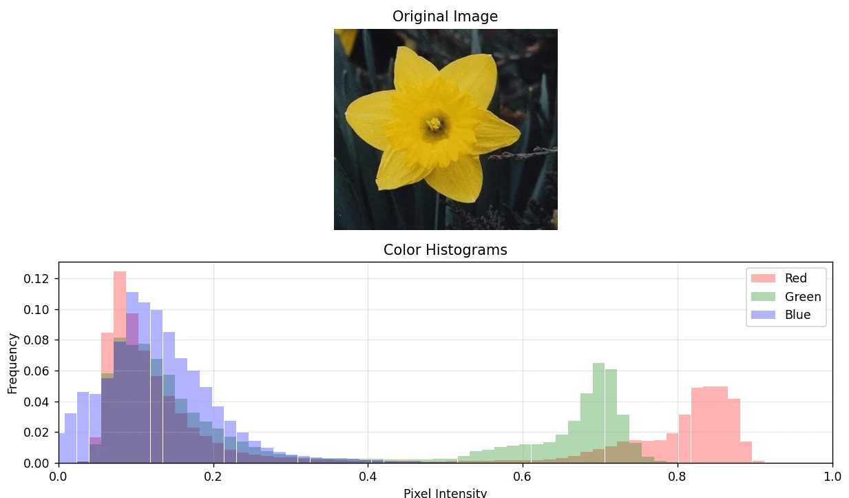
HOG describes local structure but does not explicitly preserve color. Color histograms complement it by quantizing pixel intensities separately for the red, green, and blue channels. Concatenating the three histograms produces a global representation of the image’s color distribution. The implementation uses 64 bins per channel.
Implementation
The mechanics above can be expressed in a compact implementation. The following function uses grayscale input and hard orientation-bin assignment so that the main transformations remain visible. It is an explanatory approximation rather than a complete reproduction of standard HOG.
import numpy as np
from scipy.signal import convolve2d

def hog_descriptor(image, cell_size=16, bin_count=9):
    image = np.asarray(
        image.convert('L').resize((256, 256)),
        dtype=np.float32,
    ) / 255.0

    kernel = np.array([[-1, 0, 1]], dtype=np.float32)
    gradient_x = convolve2d(image, kernel, mode='same', boundary='symm')
    gradient_y = convolve2d(image, kernel.T, mode='same', boundary='symm')
    magnitude = np.hypot(gradient_x, gradient_y)
    orientation = np.degrees(np.arctan2(gradient_y, gradient_x)) % 180

    cells_y = image.shape[0] // cell_size
    cells_x = image.shape[1] // cell_size
    histograms = np.zeros((cells_y, cells_x, bin_count))
    bin_width = 180 / bin_count

    for y in range(cells_y):
        for x in range(cells_x):
            rows = slice(y * cell_size, (y + 1) * cell_size)
            columns = slice(x * cell_size, (x + 1) * cell_size)
            bins = (orientation[rows, columns] // bin_width).astype(int)
            np.add.at(
                histograms[y, x],
                bins.ravel(),
                magnitude[rows, columns].ravel(),
            )

    descriptor = []
    for y in range(cells_y - 1):
        for x in range(cells_x - 1):
            block = histograms[y:y + 2, x:x + 2].ravel()
            descriptor.extend(block / np.sqrt(np.dot(block, block) + 1e-6))

    return np.asarray(descriptor)
For practical work, scikit-image provides an established, vectorized implementation:
import numpy as np
from skimage.feature import hog
from skimage.transform import resize

def extract_hog(image):
    image = resize(
        np.asarray(image.convert('RGB')),
        (256, 256),
        anti_aliasing=True,
    )
    return hog(
        image,
        orientations=9,
        pixels_per_cell=(16, 16),
        cells_per_block=(2, 2),
        block_norm='L2-Hys',
        channel_axis=-1,
    )
Color information can be represented independently with one normalized histogram per RGB channel:
def extract_color_histogram(image, bin_count=64):
    image = np.asarray(image.convert('RGB'))
    histograms = []

    for channel in range(3):
        histogram, _ = np.histogram(
            image[..., channel],
            bins=bin_count,
            range=(0, 256),
        )
        histogram = histogram.astype(np.float32)
        histograms.append(histogram / histogram.sum())

    return np.concatenate(histograms)
Downstream use
The two descriptors can be concatenated into a single feature vector for a conventional classifier. This final step illustrates how the feature extractors may fit into a broader pipeline. Classifier selection and performance evaluation are separate experimental questions and not discussed here.
from sklearn.ensemble import RandomForestClassifier

def extract_features(image):
    return np.concatenate([
        extract_hog(image),
        extract_color_histogram(image),
    ])

features = np.stack([extract_features(image) for image in images])
classifier = RandomForestClassifier(random_state=42)
classifier.fit(features[training_indices], labels[training_indices])
predictions = classifier.predict(features[inference_indices])
Conclusion
Implementing HOG from its individual stages shows how a useful visual representation can emerge from relatively simple operations. Gradients capture local intensity changes, cell histograms summarize their direction, and block normalization makes those measurements more stable across changes variations, for instance, in contrast. Color histograms add information that HOG intentionally leaves out, giving the combined representation access to both shape and appearance.
This pipeline is best understood as an interpretable foundation rather than a claim about state-of-the-art classification performance. Its value lies in making every transformation visible and providing a concrete basis for understanding more complex approaches to visual feature extraction.